In the 1960, a meteorologist named Edward Lorenz wanted to compare different forecasting methods to see how well they predicted the weather. So he decided to create a mathematical model of the weather system and put it on a computer. The idea of making computer models for things in real life was very new for the time, and the computer he used to run his simulation was very bulky and prone to technical issues. One day, as he was trying to rerun a previous simulation using the same initial conditions, he found that after a while, the weather in the old and new simulations was very different. Inspecting their history closer, he found that they started off very similarly, but then started to diverge quickly. He later found that the cause of his problem was a very small rounding error in his computer program, causing errors in the third decimal place - such a small error could have such large effects on the simulated weather! He had discovered chaos.
Chaos theory is the study of complex systems whose futures can rely greatly on small changes in their initial conditions. It can pop up in situations as simple as a swinging pendulum or as complex as the weather system. Chaotic systems are nonlinear and iterated - small changes grow exponentially over time and each state of the system is dependent on the previous state. The weather system is a perfect example of a chaotic system.
This idea that small changes can have very large effects in the future is called the butterfly effect, coined by Edward Lorenz. The most famous example of the butterfly effect is the idea that a small disturbance in the air on one side of the world (a butterfly flapping its wings in Brazil) can cause a very large disturbance somewhere else (a tornado in Texas).
Complex systems may seem like they act randomly, but they just have so many variables that effect their outcomes that it can be impossible to predict very far into their future. The question is, how far?
A system's predictability horizon is the amount of time it takes in a system for the effects of a small change in a model to double. For example, with Lorenz's two simulated weather models, it would be the time it took for the rounding error in the third decimal place to double. With the weather, it's about a week (this is why weather reports usually don't give specific predictions for more than a week in the future).
The "normal" way of graphing the behavior of a system is by having an axis for the time at which certain variables hold certain values. But when we draw a chaotic system this way, we get an incoherent squiggle that doesn't help us at all.
To see the structure of a chaotic system, we need to draw it using state space: instead of plotting the variables against time, have an axis for each variable. The points plotted represent a system's states. So a system with 3 variables would be plotted in 3 dimensions.
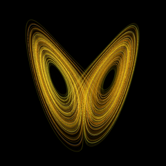
What do we get when we plot a chaotic system in state space? Depending on the initial conditions we give, a chaotic system can converge on any number of values, or not converge at all. The points on which the system may converge are called strange attractors, and they represent the average behavior of the system given the initial conditions. Eerily, the state space graph of the Lorenz weather model resembles a butterfly. In fact, its nickname is the Lorenz butterfly.
But this image of a chaotic system collapses all of its conditions at different times into one "object". What if we want to look more closely at the system at different times, and see how the variables change? The process of recording the variables at intervals and plotting them in state space is called iterated mapping. The way we do this is by using the ending conditions of one iteration as the initial conditions of another.
Now that we've learned the main concepts of chaos theory, we can start generating some lovely fractals using the Julia Set!
The concept we use the most for this is iterated mapping. Models of chaotic systems will commonly converge when you map them iteratively, and to make a nice colorful fractal, we check to see how many iterations it takes them to converge.
Before we begin, we need to understand complex numbers.
If you're already familiar with complex numbers or would rather not like to deal with variables and equations, that's ok - just jump to the explanation of my code. But for those who are interested, I explain them below...
Complex numbers have two parts - a real part and an imaginary part. The real part is just a number, like 3 or 10. The imaginary part is a number multiplied by the square root of negative one. We can write the square root of negative one using the variable \(i\). So, complex numbers take this form:
\[a + bi = a + b (\sqrt{-1})\]
You can square a complex number like so:
\[(a + bi)^2 = a^2 + 2abi + (b^2)(i^2) = (a^2 - b^2) + (2ab)i\]
To add two complex numbers, you simply add the parts:
\[(a + bi) + (c + di) = (a + c) + (b + d)i\]
Now, to generate part of the Julia set, we need to pick a complex number to start with, usually between -1 and 1. Let's pick this one:
\[-0.85 + -0.15 i\]
For every point on a coordinate plane in state space, we use the x coordinate as the real part and the y coordinate as the imaginary part of a new complex number. We then square this number and add it to the one we picked before, in this case, \(-0.85 + -0.15i\). Then we do the same thing with the result, squaring it and adding it to the number we picked. Finally, we somehow color this point based on the number it converges to.
So I made an application that draws a Julia set for a given complex number (we can call this number \(c\)) and colors the pixels in an HTML Canvas element. The source code is in JavaScript.
The first thing my program does is define some useful methods for adding and squaring complex numbers, as described earlier. We represent complex numbers using dictionaries with the labels r (real) and i (imaginary).
const addCN = ({r: r1, i: i1}, {r: r2, i: i2}) => ({r: r1+r2, i: i1+i2})
 const squareCN = ({r, i}) => ({r: (r*r) - (i*i), i: 2*r*i})
Then, we define a functuon that generates the function that will later be iterated to find the convergence value.
const makeJuliaFn = (c) => {
        return (z) => {
            return addCN( squareCN(z), c )
        }
    }
This function iterates over a given Julia function a maximum of 100 times and returns how many iterations it took to converge.
 const juliaDivergence = (jf, z, maxIter)=> {
        let i = 0
        while (i < maxIter && (Math.pow(z.r, 2) + Math.pow(z.i, 2)) < 100) {
            z = jf(z)
            i++
        }
        return i
    }
I'll skip over the insane amout of variable instantiations and simply explain what they are when we encounter them later.
Now we define a function which determines what color a pixel should be based on its convergence value, the maximum number of iterations (we set it to 100) and the color scheme we want to use. The reason we pass in the maximum number of iterations is to make the "center" of the fractal black, which just looks more aesthetic. You can make the colors change (ex. from yellow to red) as the convergence values get larger by adding some number multiplied by the convergence value to the red, green, and blue color values. This isn't an essential part of the coloring process, but it has a nice effect.
const colorsForJulia = (julia, max, scheme = "lofi") => {
        var colors = {r: 0, g: 0, b: 0, a: 255}
        var lobase = [255, 100, 0]

        switch (scheme) {
            case "lofi":
                colors.r = Math.floor(lobase[0]*Math.sin(2*Math.PI*julia/max)) + 10 * julia
                colors.g = Math.floor(lobase[1]*Math.sin(2*Math.PI*julia/max)) + 5 * julia
                colors.b = Math.floor(lobase[2]*Math.sin(2*Math.PI*julia/max))
                if (julia >= 100) { return {r: 0, g: 0, b: 0, a: 255} }
                return colors
            default:
                return colors

            // a few alternative color schemes have been cut out
        }
    }
Now that we have all the methods we need for drawing our Julia set, we have to figure out how to display it on the canvas.
First, we create the canvas using HTML:
<canvas id="julia-canv" style="border: 1px solid black;" width="550px" height="550px"></canvas>
Then we create an object to hold its width and height, and create an object of type ImageData. It's an array of arrays, and the sub-arrays hold rgba values for the color of each pixel in an image.
var idata = new ImageData(CANVAS.width, CANVAS.height, new Uint8ClampedArray(CANVAS.width * CANVAS.height * 4))
This function returns an array of arrays of color values for each pixel, based on the initial complex number we picked (here I call it the init), how far we've shifted our view in the x and y positions, how zoomed in we are, and what color scheme we want to display it with. The first thing we do is generate an x and y position for each pixel in the canvas, scaled to the zoom level. Then we get the convergence value for each pixel usng the x and y positions. Then, we create the array of arrays of color values based on the convergence values for each pixel, using the colorsForJulia function we created earlier. Finally, we return both arrays (the one with the convergence values and the one with the colors).
const setColorsJulia = (pixelData, init, shiftx, shifty, zoom, scheme) => {
    var max = 0
    var juliaValues = []
    const maxIter = 100

    const emptyDivergence = Array.from(pixelData.filter((_, i) => i % 4 == 0))

    emptyDivergence.forEach((_, i) => {
        var ypos = (Math.floor(i / canvas.width)) - (canvas.height / 2)
        var xpos = (canvas.width - i % canvas.width) - (canvas.width / 2)

        var scaledx = (xpos / canvas.width) * zoom - shiftx
        var scaledy = (ypos / canvas.height) * zoom - shifty

        var juliaVal = juliaDivergence(makeJuliaFn({r: init.r, i: init.i}), {r: scaledx, i: scaledy}, maxIter)
        max = (juliaVal > max && juliaVal < maxIter) ? juliaVal : max

        juliaValues.push(juliaVal)
    })

    const newPixelData = emptyDivergence.map((_, i) => {
        const colors = colorsForJulia(juliaValues[i], max, scheme)
        return [colors.r, colors.g, colors.b, colors.a]
    }).flat()

    return {newPixelData, juliaValues}

    }
Now we render the image on the canvas.
const render = () => {
    juliaSet = setColorsJulia(idata.data, IMAGE.spawn, IMAGE.xshift, IMAGE.yshift, IMAGE.zoom, IMAGE.colorscheme)
    idata.data.set(juliaSet.newPixelData)
    ctx.putImageData(idata, 0, 0)
}

render()
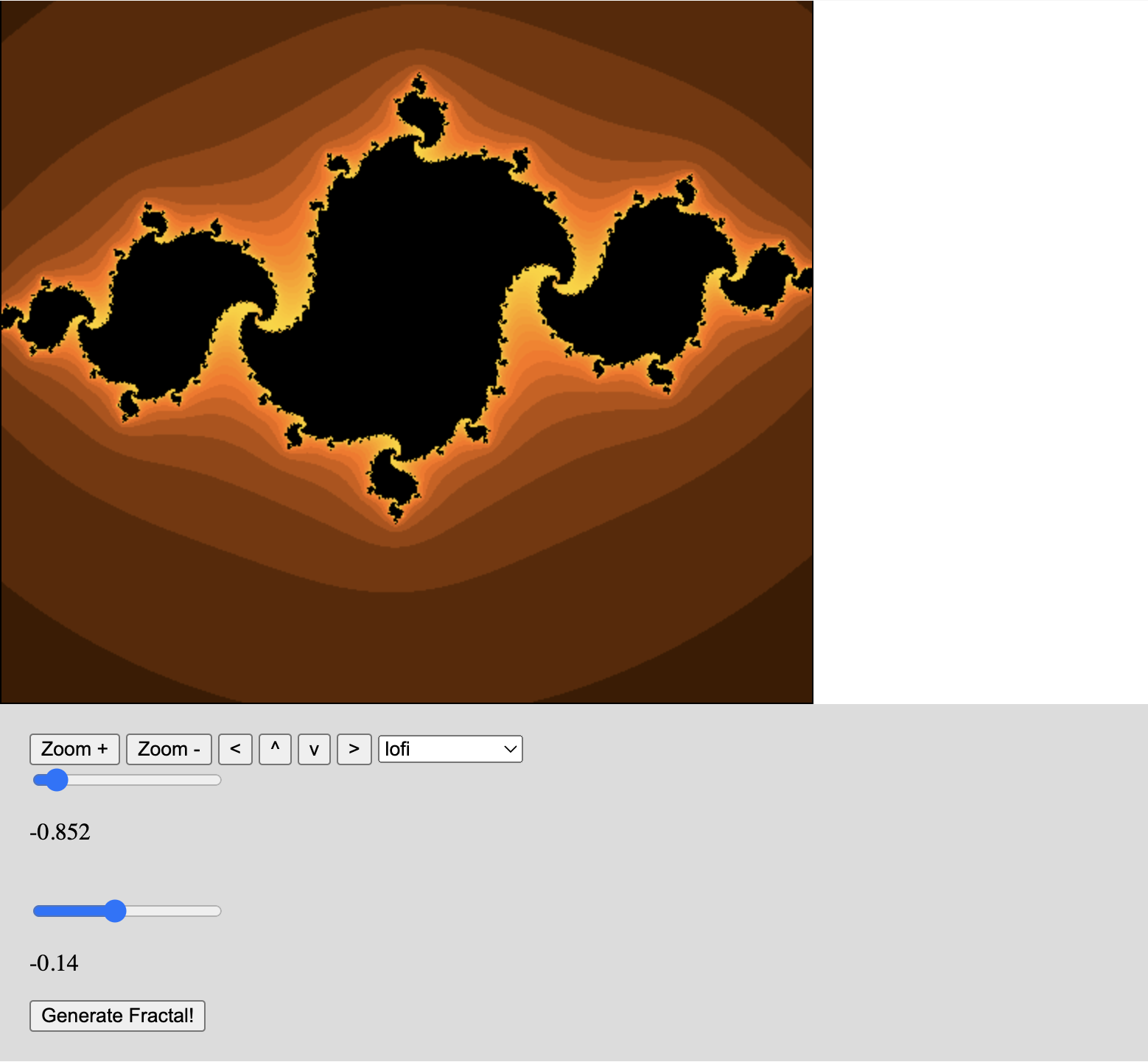
After adding some widgets on the web page and using them to control the inital value, zoom, shift, and color scheme, we get something like this: